Course
- Link
RNN
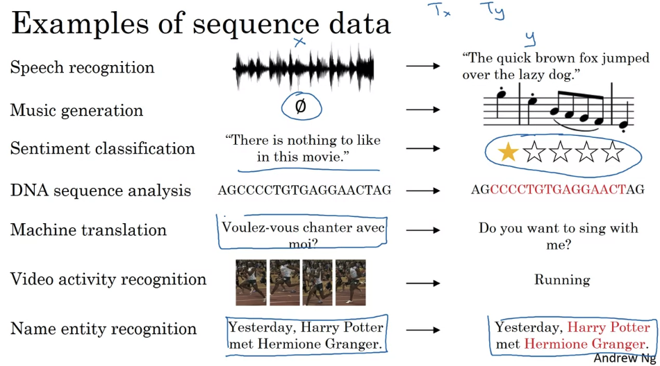
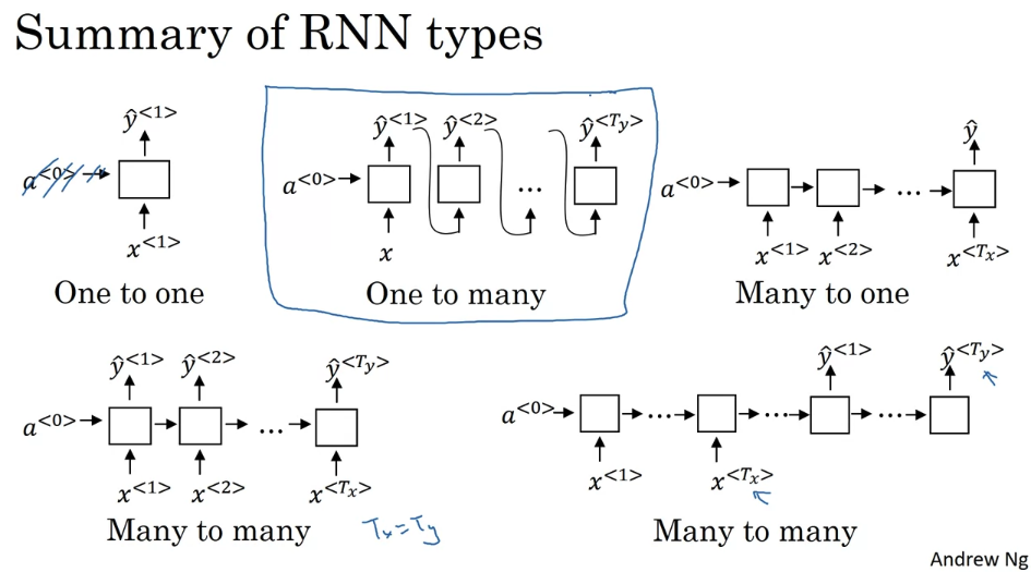
there is one-to-many. So, this was a music generation or sequenced generation as example. And then, there’s many-to-one, that would be an example of sentiment classification. Where you might want to read as input all the text with a movie review. And then, try to figure out that they liked the movie or not. There is many-to-many, so the name entity recognition, the example we’ve been using, was this where Tx is equal to Ty. And then, finally, there’s this other version of many-to-many, where for applications like machine translation, Tx and Ty no longer have to be the same.
What is language modeling?
- given any sentence, its job is to tell you what is the probability of that particular sentence, and by probability of sentence, I mean, if you were to pick up a random newspaper, open a random email, or pick a random webpage,
- what a language model does is it estimates the probability of that particular sequence of words.
Gated Recurrent Unit
- very effective solution for addressing the vanishing gradient problem and will allow your neural network to capture much longer range dependencies
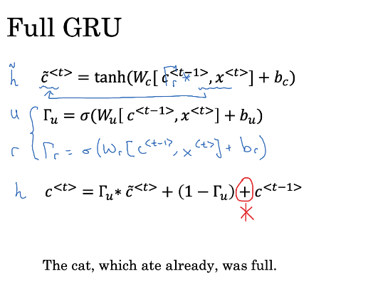
- This is another gate Gamma r. You can think of r as standing for relevance. This gate Gamma r tells you how relevant is C^t minus 1 to computing the next candidate for C^t. This gate Gamma r is computed pretty much as you expect with a new parameter matrix w _r, and then the same things as input x_t plus b_r.
- over many years, researchers have experimented with many different possible versions of how to design these units to try to have longer range connections. To try to have model long-range effects and also address vanishing gradient problems. The GRU is one of the most commonly used versions that researchers have converged to and then found as robust and useful for many different problems.
LSTM
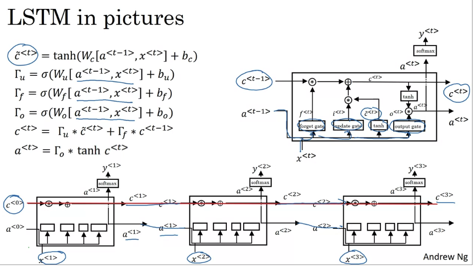
one element of this is interesting is if you hook up a bunch of these in parallel so that’s one of them and you connect them, connect these temporarily. So there’s the input x 1, then x 2, x 3. So you can take these units and just hook them up as follows where the output a for a period of time, 70 input at the next time set. And similarly for C and I’ve simplified the diagrams a little bit at the bottom. And one cool thing about this, you notice is that this is a line at the top that shows how so long as you said the forget and the update gates, appropriately, it is relatively easy for the LSTM to have some value C0 and have that be passed all the way to the right to have, maybe C3 equals C0. And this is why the LSTM as well as the GRU is very good at memorizing certain values. Even for a long time for certain real values stored in the memory cells even for many, many times steps.
peephole connection: one common variation you see of LSTMs
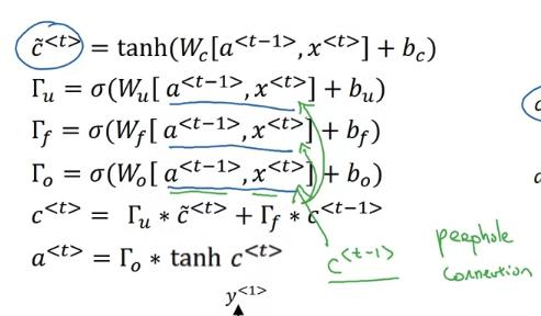
- So that’s it for the LSTM, as you can imagine, there are also a few variations on this that people use. Perhaps the most common one, is that instead of just having the gate values be dependent only on a t-1, xt. Sometimes people also sneak in there the value c t -1 as well. This is called a peephole connection.
- if you see peephole connection, what that means is that the gate values may depend not just on a t-1 but and on x t but also on the previous memory cell value. And the peephole connection can go into all three of these gates computations.
GRU vs LSTM
- the advantage of the GRU is that it’s a simpler model. And so it’s actually easier to build a much bigger network only has two gates, so computation runs a bit faster so it scales the building, somewhat bigger models. But the LSTM is more powerful and more flexible since there’s three gates instead of two. If you want to pick one to use, I think LSTM has been the historically more proven choice. So if you had to pick one, I think most people today will still use the LSTM as the default first thing to try.
Bidirectional RNN
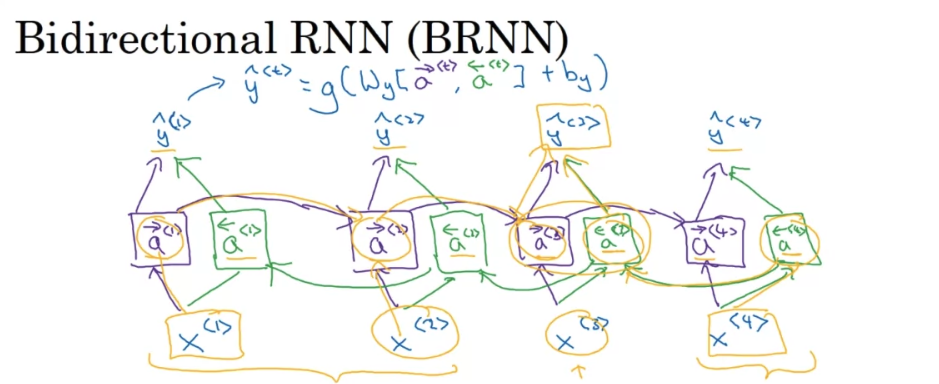
- you can have a model that uses RNN, or GRU, LSTM, and is able to make predictions anywhere even in the middle of the sequence, but take into account information potentially from the entire sequence. The disadvantage of the bidirectional RNN is that, you do need the entire sequence of data before you can make predictions anywhere. So, for example, if you’re building a speech recognition system then BRNN will let you take into account the entire speech other friends. But if you use this straightforward implementation, you need to wait for the person to stop talking to get the entire utterance before you can actually process it, and make a speech recognition prediction. So the real time speech recognition applications, there is somewhat more complex models as well rather than just using the standard by the rational RNN as you’re seeing here. But for a lot of natural language processing applications where you can get the entire sentence all at the same time, the standard BRNN and algorithm is actually very effective.
NLP
word embeddings
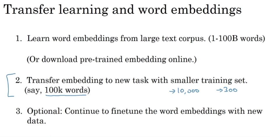
- this is how you can carry out transfer learning using word embeddings. Step 1 is to learn word embeddings from a large text corpus, a very large text corpus or you can also download pre-trained word embeddings online. There are several word embeddings that you can find online under very permissive licenses. And you can then take these word embeddings and transfer the embedding to new task, where you have a much smaller labeled training sets. And use this, let’s say, 300 dimensional embedding, to represent your words. One nice thing also about this is you can now use relatively lower dimensional feature vectors. So rather than using a 10,000 dimensional one-hot vector, you can now instead use maybe a 300 dimensional dense vector. Although the one-hot vector is fast and the 300 dimensional vector that you might learn for your embedding will be a dense vector.
- And then, finally, as you train your model on your new task, on your named entity recognition task with a smaller label data set, one thing you can optionally do is to continue to fine tune, continue to adjust the word embeddings with the new data. In practice, you would do this only if this task 2 has a pretty big data set. If your label data set for step 2 is quite small, then usually, I would not bother to continue to fine tune the word embeddings.
Word2Vec
- you saw how the Skip-Gram model allows you to construct a supervised learning task. So we map from context to target and how that allows you to learn a useful word embedding. But the downside of that was the Softmax objective was slow to compute.
Negative Sampling
- technique is called negative sampling because what you’re doing is, you have a positive example, the orange and then juice. And then you will go and deliberately generate a bunch of negative examples, negative samplings, hence, the name negative sampling, with which to train four more of these binary classifiers. And on every iteration, you choose four different random negative words with which to train your algorithm on.
- To summarize, you’ve seen how you can learn word vectors in a Softmax classier, but it’s very computationally expensive. And in this video, you saw how by changing that to a bunch of binary classification problems, you can very efficiently learn words vectors. And if you run this algorithm, you will be able to learn pretty good word vectors. Now of course, as is the case in other areas of deep learning as well, there are open source implementations. And there are also pre-trained word vectors that others have trained and released online under permissive licenses. And so if you want to get going quickly on a NLP problem, it’d be reasonable to download someone else’s word vectors and use that as a starting point.
Attention
greedy search
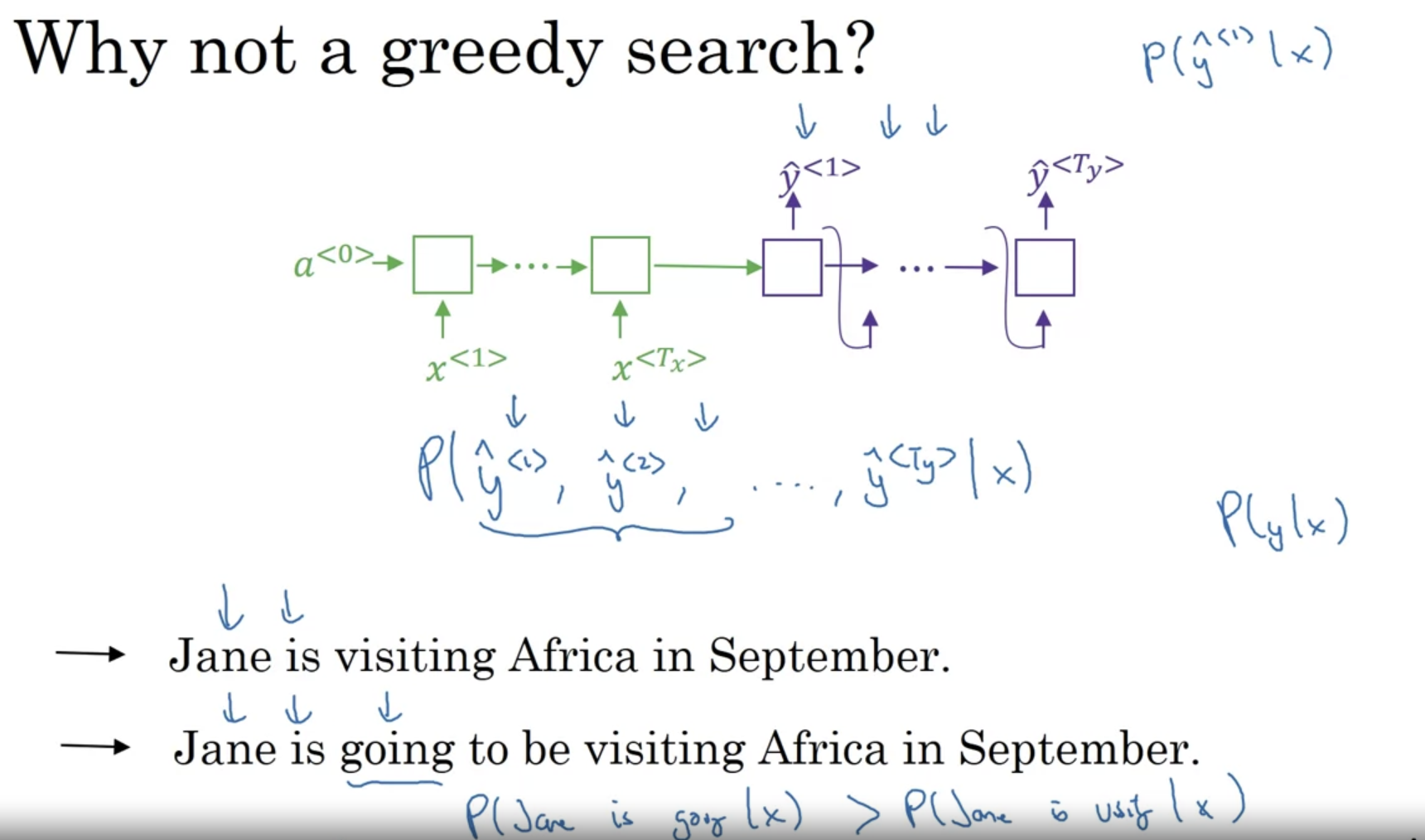
- greedy search is an algorithm from computer science which says to generate the first word just pick whatever is the most likely first word according to your conditional language model. Going to your machine translation model and then after having picked the first word, you then pick whatever is the second word that seems most likely, then pick the third word that seems most likely.
- it turns out that the greedy approach, where you just pick the best first word, and then, after having picked the best first word, try to pick the best second word, and then, after that, try to pick the best third word, that approach doesn’t really work. Because ‘going’ is much more common word than ‘visiting’ so if you use greedy search to translate, ‘going’ has higher possibility to be chosen. However the best choice of translation is the first sentence.
- one major difference between this and the earlier language modeling problems is rather than wanting to generate a sentence at random, you may want to try to find the most likely English sentence, most likely English translation. But the set of all English sentences of a certain length is too large to exhaustively enumerate. So, we have to resort to a search algorithm.
Beam Search
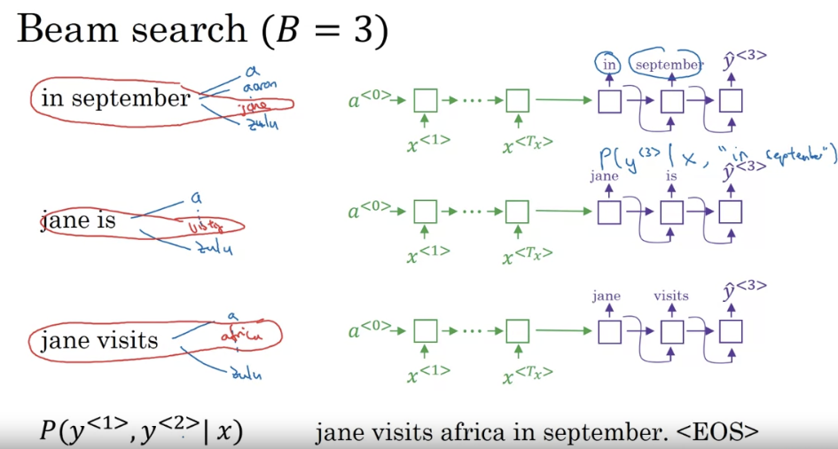
- with a beam of three being searched considers three possibilities at a time. Notice that if the beam width was said to be equal to one, say cause there’s only one, then this essentially becomes the greedy search algorithm which we had discussed in the last video but by considering multiple possibilities say three or ten or some other number at the same time beam search will usually find a much better output sentence than greedy search.
- how do you choose the beam width? Share the pros and cons of setting beam to be very large versus very small. If the beam width is very large, then you consider a lot of possibilities and so you tend to get a better result because you’re consuming a lot of different options, but it will be slower. The memory requirements will also grow and also be computationally slower. Whereas if you use a very small beam width, then you get a worse result because you are just keeping less possibilities in mind as the algorithm is running, but you get a result faster and the memory requirements will also be lower.
- I would say try out a variety of values of beam as see what works for your application, but when beam is very large, there is often diminishing returns. For many applications, I would expect to see a huge gain as you go from beam of one, which is basically research to three to maybe 10, but the gains as you go from the thousands of thousand beam width might not be as big.
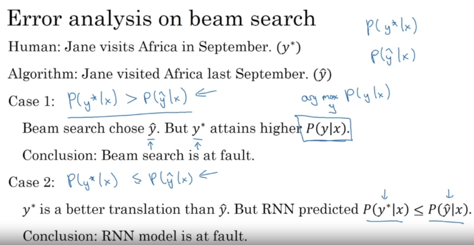
- even though y* is a better translation, the RNN ascribed y* in lower probability than the inferior translation. So in this case, I will say the RNN model is at fault. So the error analysis process looks as follows. You go through the development set and find the mistakes that the algorithm made in the development set.
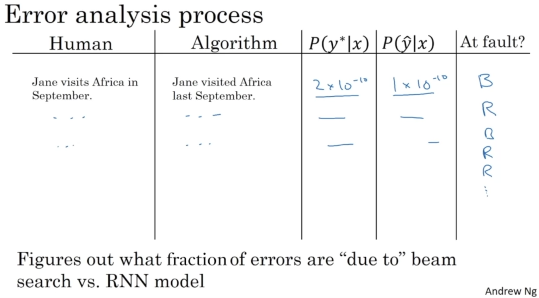
- through this process, you can then carry out error analysis to figure out what fraction of errors are due to beam search versus the RNN model. if you find that beam search is responsible for a lot of errors, then maybe is we’re working hard to increase the beam width. Whereas in contrast, if you find that the RNN model is at fault, then you could do a deeper layer of analysis to try to figure out if you want to add regularization, or get more training data, or try a different network architecture, or something else.
Bleu score
- One of the challenges of machine translation is that, given a French sentence, there could be multiple English translations that are equally good translations of that French sentence. So how do you evaluate a machine translation system if there are multiple equally good answers, unlike, say, image recognition where there’s one right answer? You just measure accuracy. If there are multiple great answers, how do you measure accuracy? The way this is done conventionally is through something called the BLEU score.
Attention Model
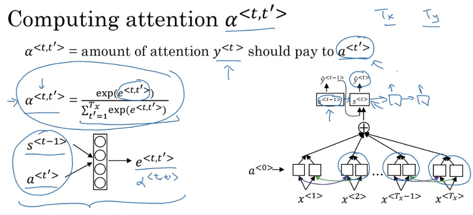
- it’s for long sentece translation because encoder-decoder algorithm is hard to remember whole sentence if it is too long.
Speech Recognition
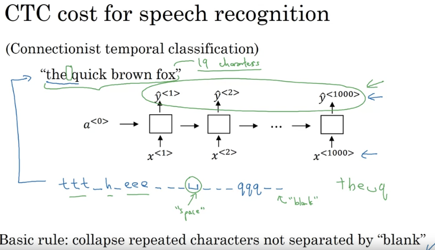
- how do you build a speech recognition system? One method that seems to work well is to use the CTC cost for speech recognition. CTC stands for Connection is Temporal Classification
- the basic rule for the CTC cost function is to collapse repeated characters not separated by “blank”. So, to be clear, I’m using this underscore to denote a special blank character and that’s different than the space character
Trigger word system
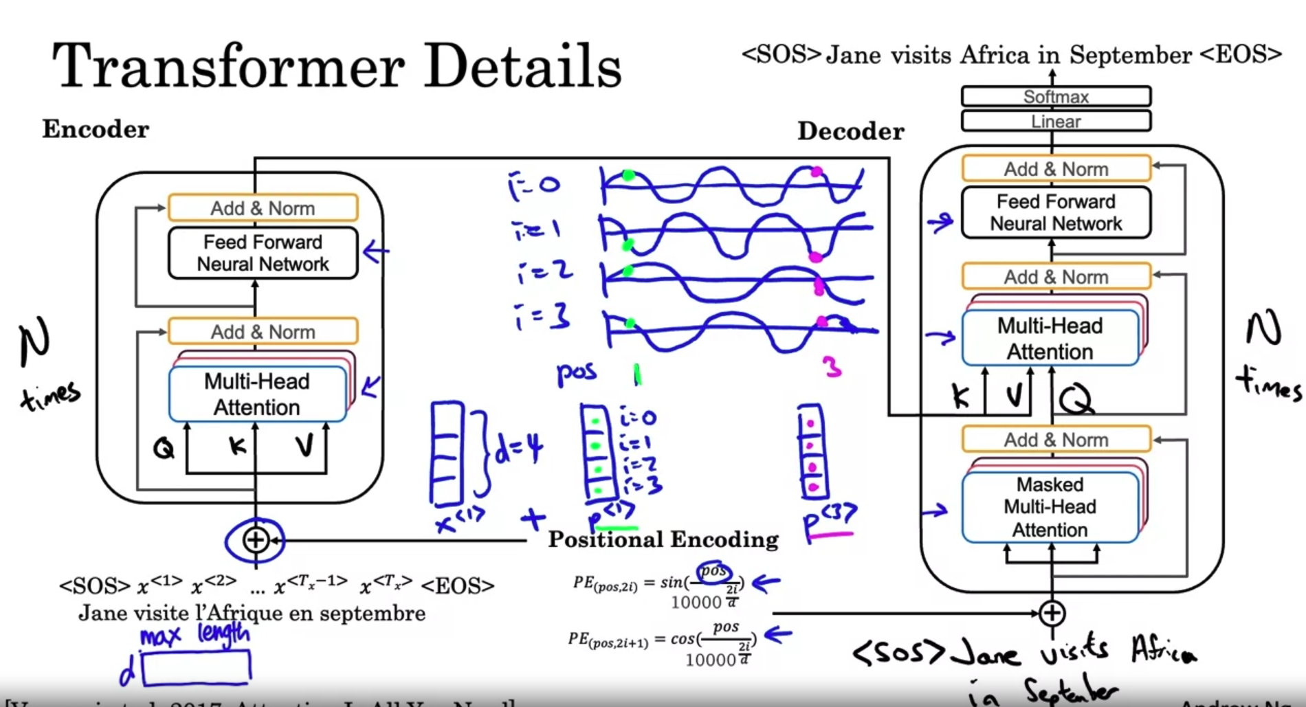
Transformer
The major innovation of the transformer architecture is combining the use of attention based representations and a CNN convolutional neural network style of processing.
Self Attention
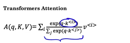
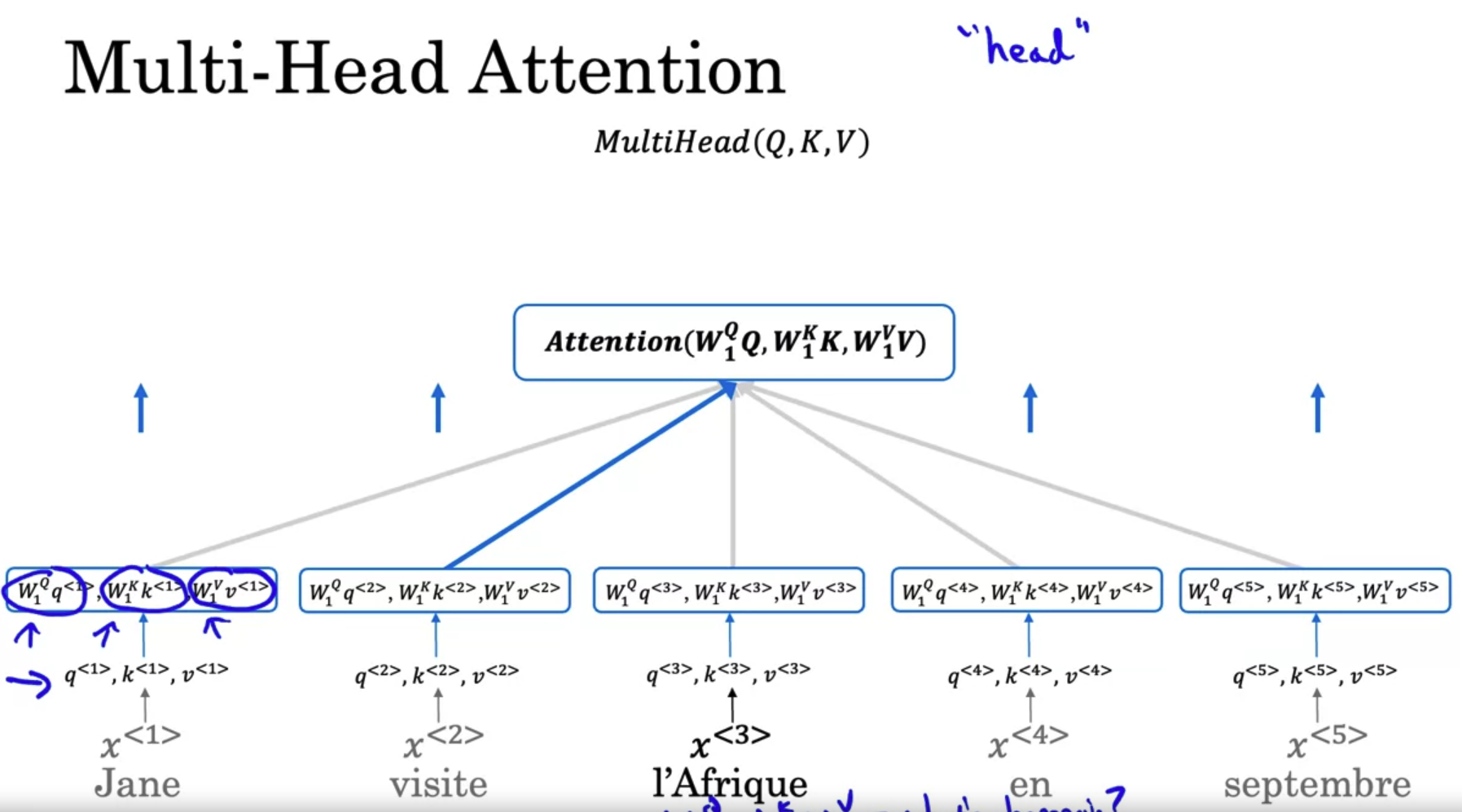
- the main difference is that for every word, say for l’Afrique, you have three values called the query, key, and value. These vectors are the key inputs to computing the attention value for each words.
- what are these query key and value vectors supposed to do? They were indeed using a loose analogy to a concert and databases where you can have queries and also key-value pairs.
- To recap, associated with each of the five words you end up with a query, a key, and a value. The query lets you ask a question about that word, such as what’s happening in Africa. The key looks at all of the other words, and by the similarity to the query, helps you figure out which words gives the most relevant answer to that question. In this case, visite is what’s happening in Africa, someone’s visiting Africa. Then finally, the value allows the representation to plug in how visite should be represented within A^3, within the representation of Africa. This allows you to come up with a representation for the word Africa that says this is Africa and someone is visiting Africa.
multi-head attention
Transformer