Course
- Link
CNN
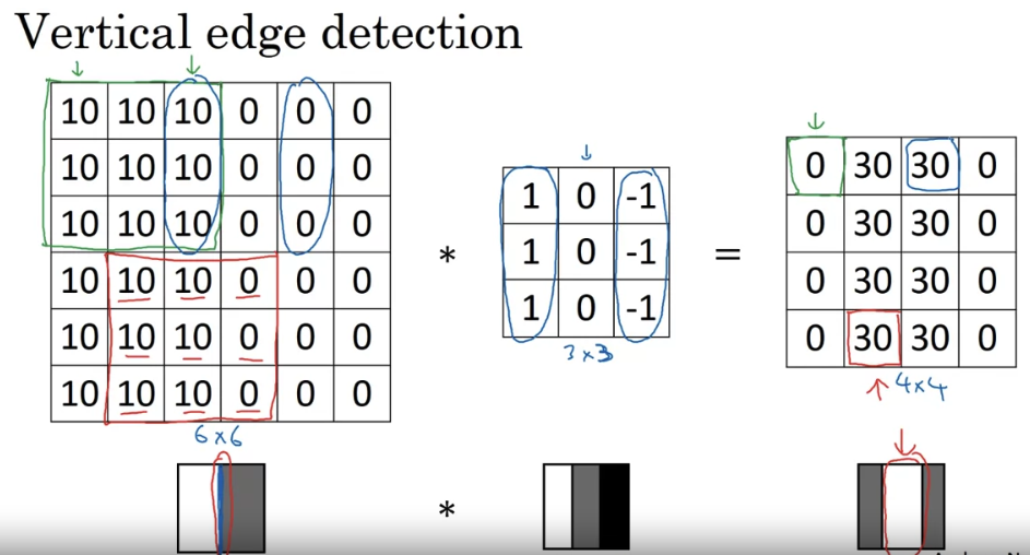
- By convention, in machine learning, we usually do not bother with this flipping operation. Technically this operation is maybe better called cross-correlation. But most of the deep learning literature just causes the convolution operator.
CNN Case
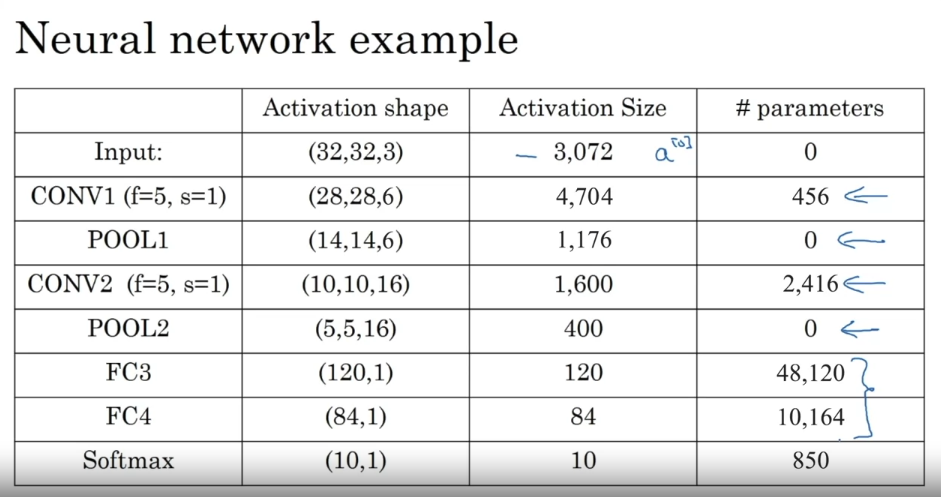
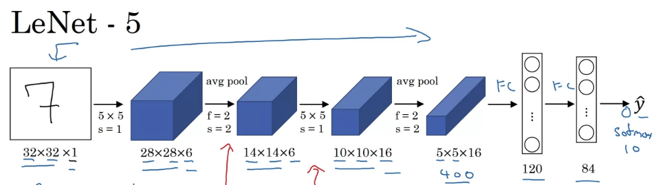
LeNet-5
AlexNet
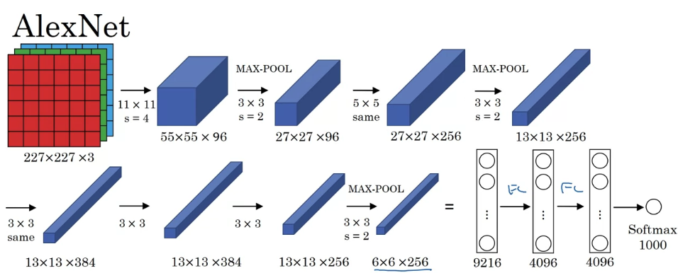
- this neural network actually had a lot of similarities to LeNet, but it was much bigger. So whereas the LeNet-5 from previous slide had about 60,000 parameters, this AlexNet that had about 60 million parameters. And the fact that they could take pretty similar basic building blocks that have a lot more hidden units and training on a lot more data, they trained on the image that dataset that allowed it to have a just remarkable performance. Another aspect of this architecture that made it much better than LeNet was using the relu activation function.
VGG-16
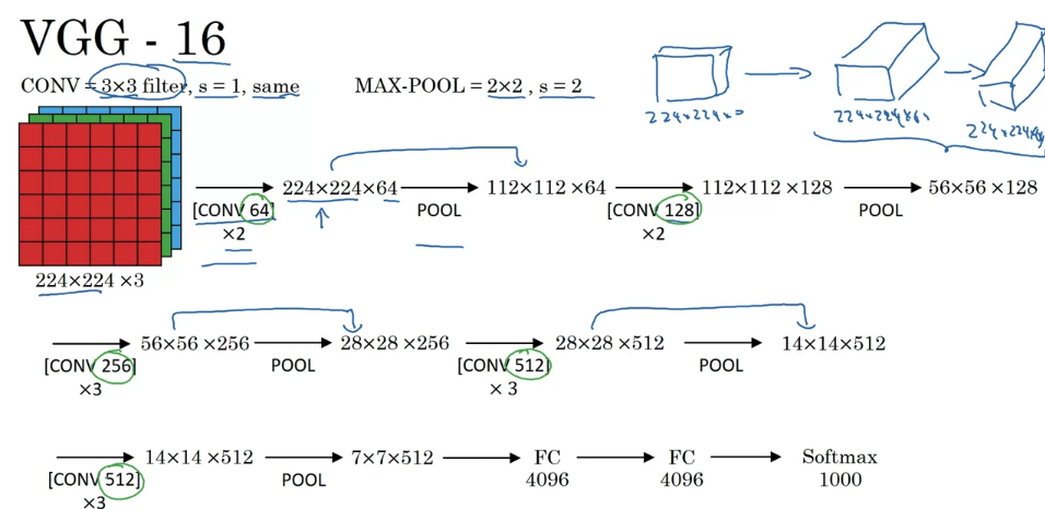
- the 16 in the VGG-16 refers to the fact that this has 16 layers that have weights. And this is a pretty large network, this network has a total of about 138 million parameters. And that’s pretty large even by modern standards.
ResNet
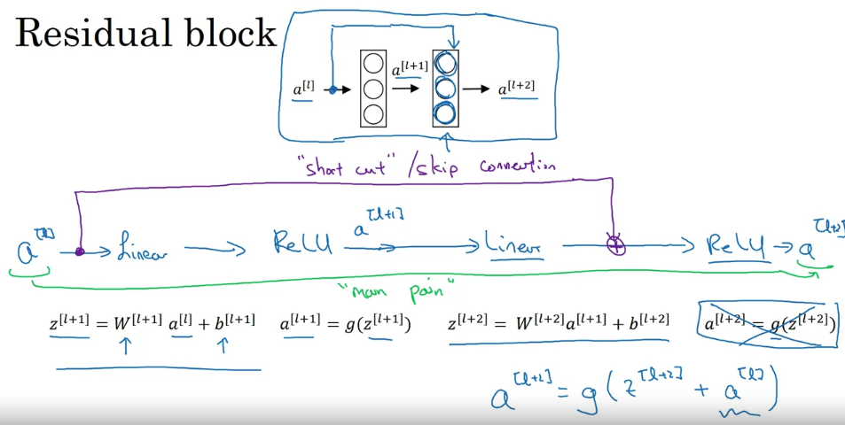
- Residual block: using residual blocks allows you to train much deeper neural networks. And the way you build a ResNet is by taking many of these residual blocks, blocks like these, and stacking them together to form a deep network.
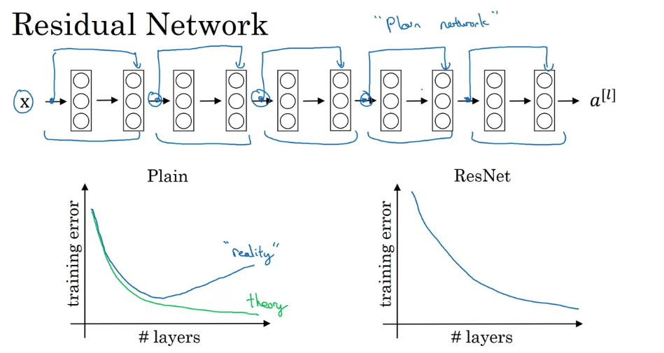
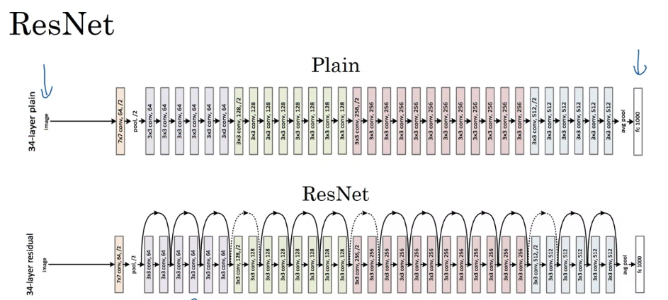
- the theory, in theory, having a deeper network should only help. But in practice or in reality, having a plain network, so no ResNet, having a plain network that is very deep means that all your optimization algorithm just has a much harder time training. And so, in reality, your training error gets worse if you pick a network that’s too deep. But what happens with ResNet is that even as the number of layers gets deeper, you can have the performance of the training error kind of keep on going down. Even if we train a network with over a hundred layers.
Network in network(1 X 1 Convolutions)
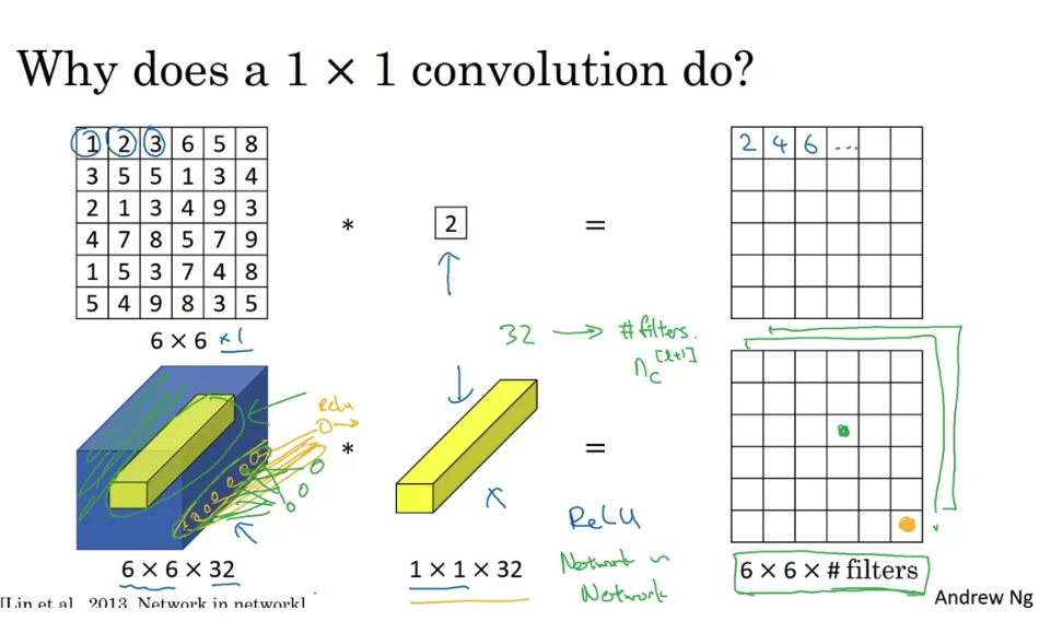
- one way to think about the 32 numbers you have in this one, a one by 32 filter is as if you have one neuron that is taking us input 32 numbers. Multiplying each of these 32 numbers in one slice in the same position, height, and width, but these 32 different channels, multiplying them by 32 weights.
- One way to think about a one-by-one convolution is that it is basically having a fully connected neural network that applies to each of the 62 different positions.
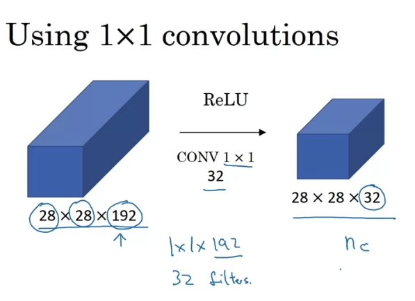
- shrinking channels
Inception Network
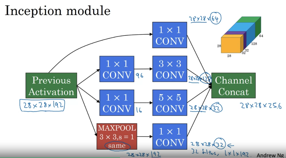
- what the inception network does, is, more or less, put a lot of these modules together.
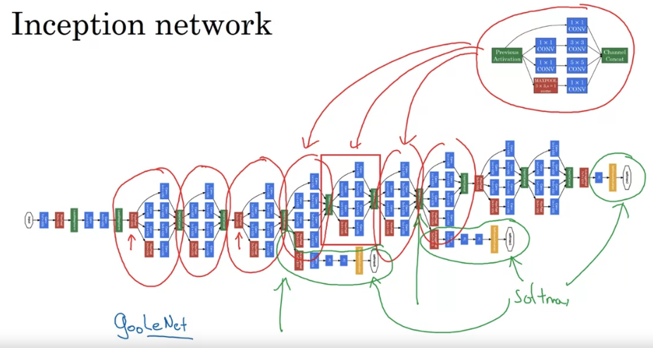
- It turns out that there’s one last detail to the inception network if we read the optional research paper. Which is that there are these additional side-branches that I just added. So what do they do? Well, the last few layers of the network is a fully connected layer followed by a softmax layer to try to make a prediction. What these side branches do is it takes some hidden layer and it tries to use that to make a prediction. So this is actually a softmax output and so is that. And this other side branch, again it is a hidden layer passes through a few layers like a few connected layers. And then has the softmax try to predict what’s the output label. And you should think of this as maybe just another detail of the inception that’s worked. But what is does is it helps to ensure that the features computed. Even in the heading units, even at intermediate layers. That they’re not too bad for protecting the output cause of a image. And this appears to have a regularizing effect on the inception network and helps prevent this network from overfitting.
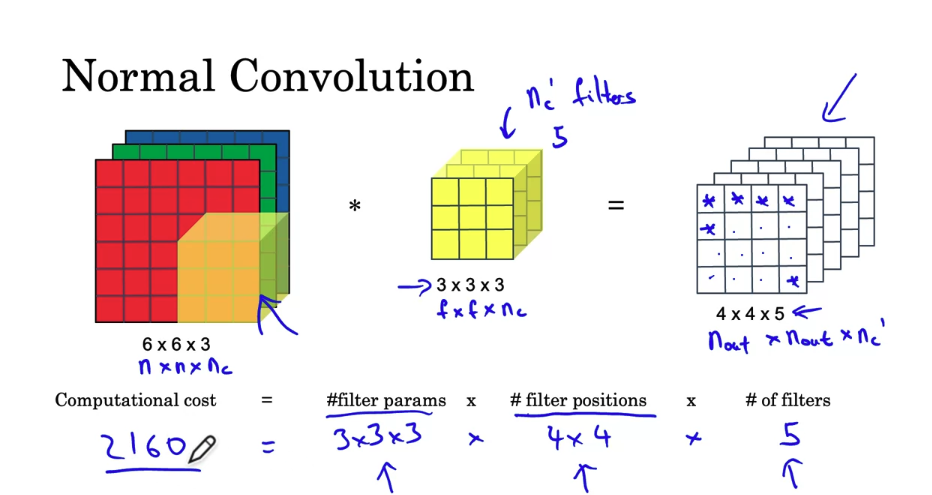
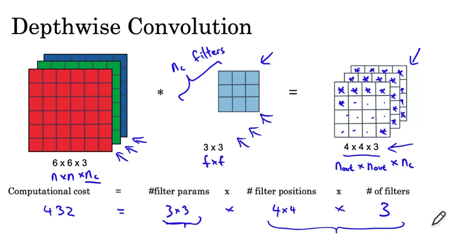
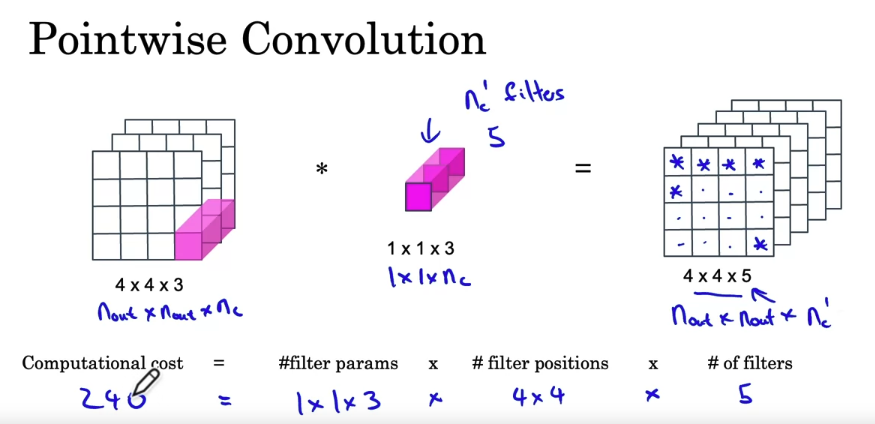
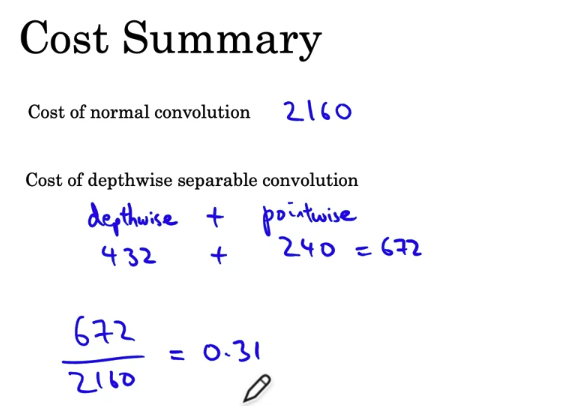
Depth-wise seperable convolution
- you’ll learn about MobileNets, which is another foundational convolutional neural network architecture used for computer vision. Using MobileNets will allow you to build and deploy new networks that work even in low compute environment, such as a mobile phone.
MobileNet
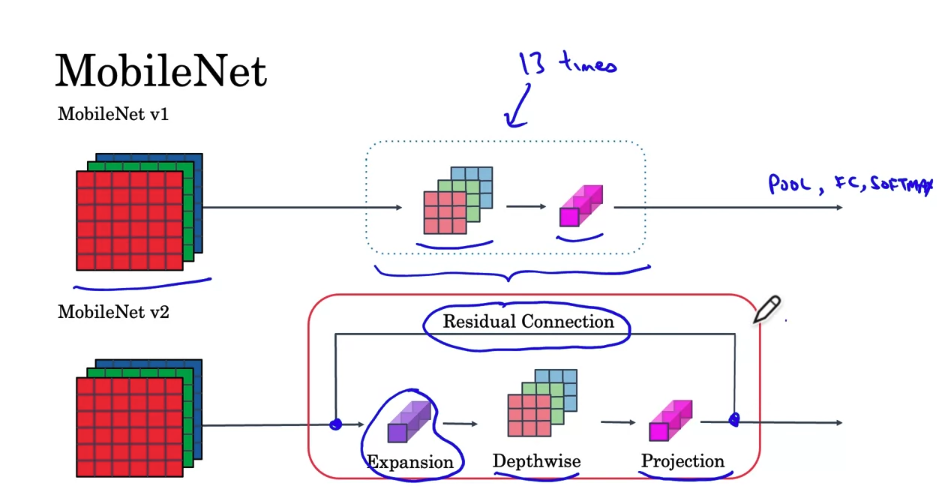
- In MobileNet v2, there are two main changes. One is the addition of a residual connection. This is just a residual connections that you learned about in the ResNet videos. This residual connection or skip connection, takes the input from the previous layer and sums it or passes it directly to the next layer, does allow ingredients to propagate backward more efficiently. The second change is that it also as an expansion layer, which you learn more about on the next slide, before the depthwise convolution, followed by the pointwise convolution, which we’re going to call projection in a point-wise convolution.
- The block with red line is called bottleneck block
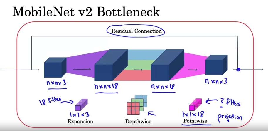
- why do we meet these bottleneck blocks? It turns out that the bottleneck block accomplishes two things, One, by using the expansion operation, it increases the size of the representation within the bottleneck block. This allows the neural network to learn a richer function. There’s just more computation over here. But when deploying on a mobile device, on edge device, you will often be heavy memory constraints. The bottleneck block uses the pointwise convolution or the projection operation in order to project it back down to a smaller set of values, so that when you pass this the next block, the amount of memory needed to store these values is reduced back down.
EfficientNet
- With MobileNet, you’ve learned how to build more computationally efficient layers, and with EfficientNet, you can also find a way to scale up or down these neural networks based on the resources of a device you may be working on.
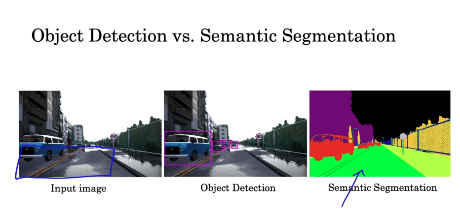
Object Detection
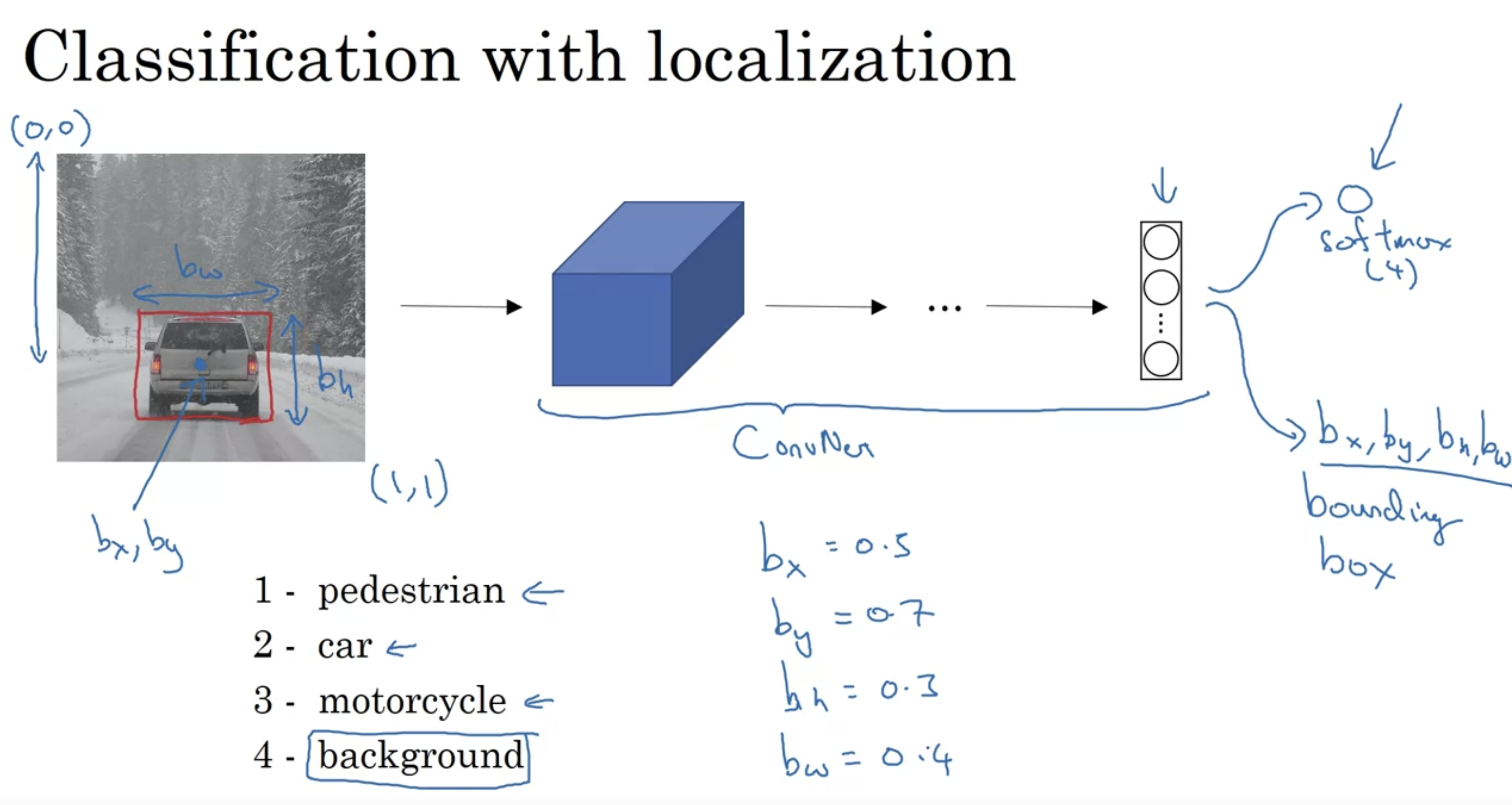
- in this example the ideal bx might be about 0.5 because this is about halfway to the right to the image. by might be about 0.7 since it’s about maybe 70% to the way down to the image. bh might be about 0.3 because the height of this red square is about 30% of the overall height of the image. And bw might be about 0.4 let’s say because the width of the red box is about 0.4 of the overall width of the entire image.
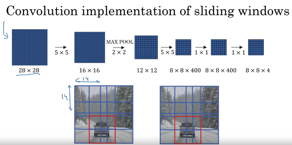
- to implement sliding windows, previously, what you do is you crop out a region. Let’s say this is 14 by 14 and run that through your convnet and do that for the next region over, then do that for the next 14 by 14 region, then the next one, then the next one, then the next one, then the next one and so on, until hopefully that one recognizes the car. But now, instead of doing it sequentially, with this convolutional implementation that you saw in the previous slide, you can implement the entire image, all maybe 28 by 28 and convolutionally make all the predictions at the same time by one forward pass through this big convnet and hopefully have it recognize the position of the car. So that’s how you implement sliding windows convolutionally and it makes the whole thing much more efficient.
Application
Face recognition
One of the challenges of face recognition is that you need to solve the one-shot learning problem. What that means is that for most face recognition applications you need to be able to recognize a person given just one single image, or given just one example of that person’s face. And, historically, deep learning algorithms don’t work well if you have only one training example.
to input two faces and tell you how similar or how different they are. A good way to do this is to use a Siamese network.
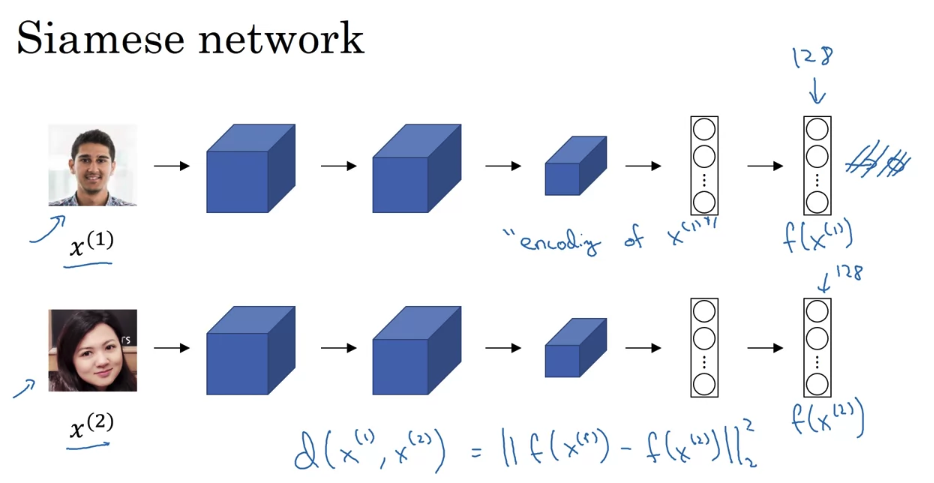
this idea of running two identical, convolutional neural networks on two different inputs and then comparing them, sometimes that’s called a Siamese neural network architecture.
Neural Style Transfer
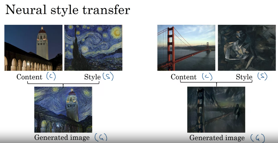
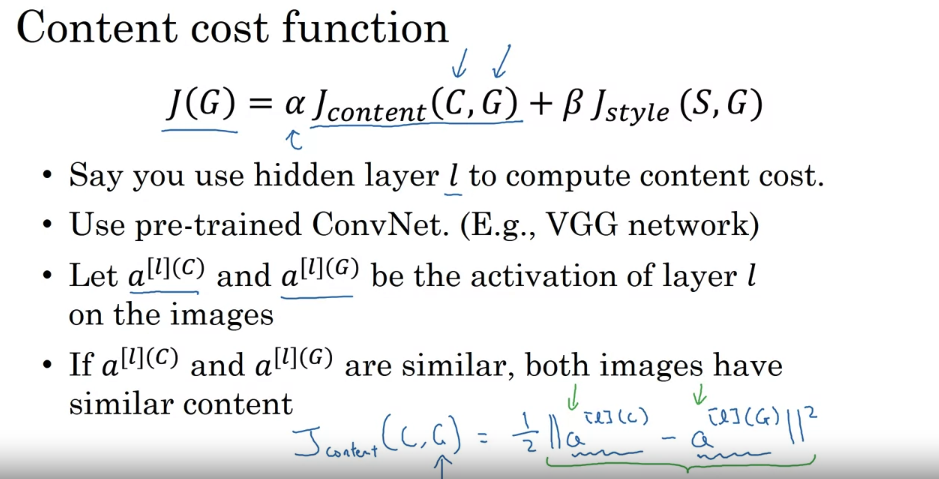
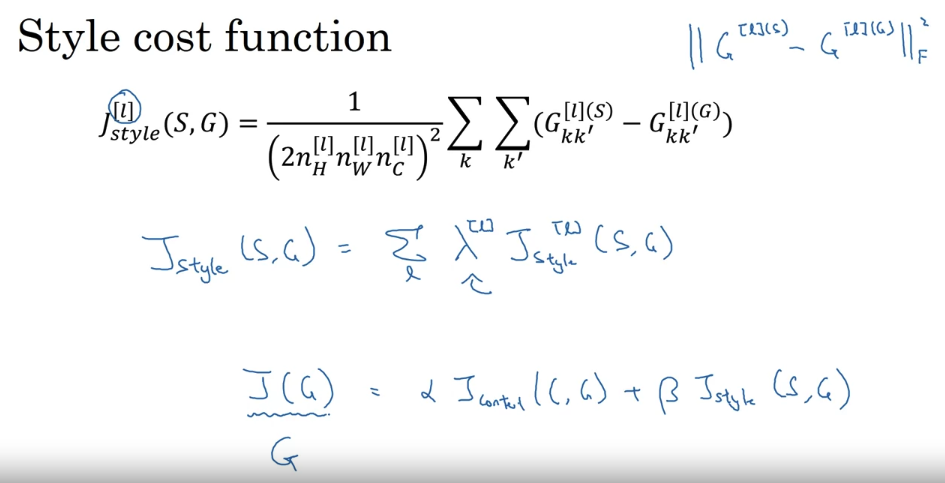
- just to wrap this up, you can now define the overall cost function as alpha times the content cost between c and G plus beta times the style cost between s and G and then just create in the sense or a more sophisticated optimization algorithm if you want in order to try to find an image G that normalize, that tries to minimize this cost function j of G. And if you do that, you can generate pretty good looking neural artistic and if you do that you’ll be able to generate some pretty nice novel artwork.