1. K-Means
- It can be used for easy, concise, and large data.
- If the number of features becomes too large with distance-based algorithms, the performance of clustering is degraded.
- Therefore, in some cases, it is applied with reducing dimensions using PCA
- In addition, since it is an iterative algorithm, it is a model that is quite sensitive to outliers and learning execution time could slow down when the number of iterations increases rapidly.
- The K-means API in Scikit-learn provides the following key parameters.
- n_clusters : As the number of clusters defined in advance, it defines how many clusters K-means will cluster into, that is, the “K” value.
- init : It is a method of initially setting the coordinates of the cluster center point and is usually set in the ‘k-means++’ method. It is used because setting it in a random way can lead to out-of-the-way results.
- max_iter : It is to set the number of iterations. If clustering is completed before the set number of times is reached, it ends in the middle even if the number of iterations is not filled.
- The following are attribute values returned by the K-means API provided by Skikit-learn. In other words, these are values returned by K-means after performing all clustering.
labels_ : Returns the cluster label to which each individual data point belongs.
(However, keep in mind that this label value is not mapped to the same value as the label value of the actual original data!)cluster_centers_ : After clustering into K clusters, the coordinates of the center points of each K cluster are returned. Using this, the center point coordinates can be visualized.
1
2
3
4
5
6
7
8
9
10
11
12
13
14
15
16
17
18
19
20
21
22
23
24
25
26
from sklearn.datasets import make_blobs
# X에는 데이터, y에는 클러스터링 된 label값 반환
X, y = make_blobs(n_samples=200, n_features=2, centers=3,
cluster_std=0.8, random_state=1)
print(X.shape, y.shape)
# y Target값 분포 확인
# return_counts=True 추가하면 array요소마다 value_counts()해줌
unique, counts = np.unique(y, return_counts=True)
# 클러스터링용으로 생성한 데이터 데이터프레임으로 만들기
cluster_df = pd.DataFrame(data=X, columns=['ftr1','ftr2'])
cluster_df['target'] = y
cluster_df.head()
# 생성 데이터포인트들 시각화해보기
target_lst = np.unique(y)
markers = ['o','s','^','P','D']
for target in target_lst:
target_cluster = cluster_df[cluster_df['target']==target]
plt.scatter(x=target_cluster['ftr1'],
y=target_cluster['ftr2'],
edgecolor='k', marker=markers[target])
plt.show()Let’s look at the distribution of individual data made with the make_blobs function that creates a clustering dataset.
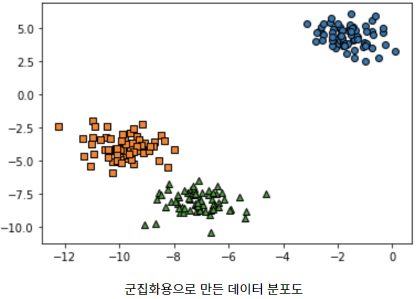
Now, let’s apply K-means to the above data to visualize the coordinates of the center points of each cluster.
1
2
3
4
5
6
7
8
9
10
11
12
13
14
15
16
17
18
19
20
21
22
23
24
25
26
27
28
29
30
31
32
33
# K-means 클러스터링 수행하고 개별 클러스터 중심을 시각화
# 1.K-means 할당
kmeans = KMeans(n_clusters=3, init='k-means++',
max_iter=200, random_state=12)
# X는 cluster_df의 feature array임.
cluster_labels = kmeans.fit_predict(X)
cluster_df['kmeans_label'] = cluster_labels
# 2.K-means속성의 cluster_centers_는 개별 클러스터의 중심 위치 좌표를 반환
centers = kmeans.cluster_centers_
unique_labels = np.unique(cluster_labels)
markers = ['o','s','^','P']
# 3. label별로 루프돌아서 개별 클러스터링의 중심 시각화
for label in unique_labels:
label_cluster = cluster_df[cluster_df['kmeans_label'] == label]
# 각 클러스터의 중심 좌표 할당
center_x_y = centers[label]
# 각 클러스터 데이터들 시각화
plt.scatter(x=label_cluster['ftr1'],
y=label_cluster['ftr2'],
marker=markers[label])
# 각 클러스터의 중심 시각화
# 중심 표현하는 모형 설정
plt.scatter(x=center_x_y[0], y=center_x_y[1], s=200,
color='white', alpha=0.9, edgecolor='k',
marker=markers[label])
# 중심 표현하는 글자 설정
plt.scatter(x=center_x_y[0], y=center_x_y[1], s=70,
color='k', edgecolor='k',
marker='$%d$' % label)# label값에 따라 숫자로 표현한다는 의미
plt.show()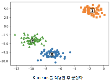
- The K-means API in Scikit-learn provides the following key parameters.
2. GMM
It is a parametric model and is a representative clustering model using EM algorithms.
It is to estimate the probability that individual data belongs to a specific normal distribution under the assumption that they belong to a Gaussian distribution.
n_components is main parameter of the API provided by Scikit-learn which refers to the number of clustering predefined
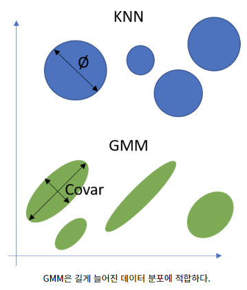
- GMM has a particularly well-applied data distribution, which is mainly easy to apply to elliptical elongated data distributions
1
2
3
4
5
6
7
8
9
10
11
12
13
14
15
16
17
18
19
20
21
22
23
24
25
26
from sklearn.datasets import load_iris
from sklearn.cluster import KMeans
import matplotlib.pyplot as plt
import numpy as np
import pandas as pd
%matplotlib inline
iris = load_iris()
feature_names = ['sepal_length','sepal_width','petal_length','petal_width']
# 보다 편리한 데이타 Handling을 위해 DataFrame으로 변환
irisDF = pd.DataFrame(data=iris.data, columns=feature_names)
irisDF['target'] = iris.target
# GMM 적용
from sklearn.mixture import GaussianMixture
# n_components로 미리 군집 개수 설정
gmm = GaussianMixture(n_components=3, random_state=42)
gmm_labels = gmm.fit_predict(iris.data)
# GMM 후 클러스터링 레이블을 따로 설정
irisDF['gmm_cluster'] = gmm_labels
# 실제 레이블과 GMM 클러스터링 후 레이블과 비교해보기(두 레이블 수치가 동일해야 똑같은 레이블 의미 아님!)
print(irisDF.groupby('target')['gmm_cluster'].value_counts())The result values are as follows, where target is the label of the actual original data, and gmm_cluster is the label of clustering after clustering.
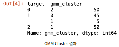
To interpret the above results, all of the labels with a target of 0 were clustered into a clustering label of 2. It is 100% well clustered. On the other hand, among the labels with a target of 1, there are 45 clusters with 0 and 5 clusters with 1, so there are 5 incorrectly clustered data.